Week 38: Sea Creatures

Over the weeks I have only done blog posts for TidyTuesday. Today for week 38, I am going to present my blog post in a presentation. This presentation does not include plots, but the code only. Therefore, I am putting the plots here.

{{% tweet "1074965237231697921" %}}

IOS slide Presentation

• Rmarkdown for the same presentation

Below is the content from the presentation, but I have included the plots.

#load the packages
library(readr)
library(lubridate)
library(tidyverse)
library(magrittr)
library(ggthemr)
library(stringr)

Introduction

• 2194 observations.
• 21 variables.
• Data : Cetacean Data
• Read : The Pudding Article
• About : Big Fish in the Sea.

Packages Used

• readr
• lubridate
• tidyverse
• magrittr
• ggthemr
• stringr

#load the data
SeaCreature <- read_csv("allCetaceanData.csv", 
                         col_types = cols(X1 = col_skip()))
attach(SeaCreature)

# loading theme
ggthemr("flat dark")

Species vs Sex vs BirthYear (code)

Plot1<-ggplot(SeaCreature,aes(x=species,y=birthYear,color=sex))+
       geom_jitter()+
       coord_flip()+
       theme(axis.text.x =element_text(angle = 90, hjust = 1))+
       ggtitle("Species and Sex over their BirthYear")+
       ylab("Birth Year")+
       xlab("Species")+ 
       legend_bottom()  

Plot1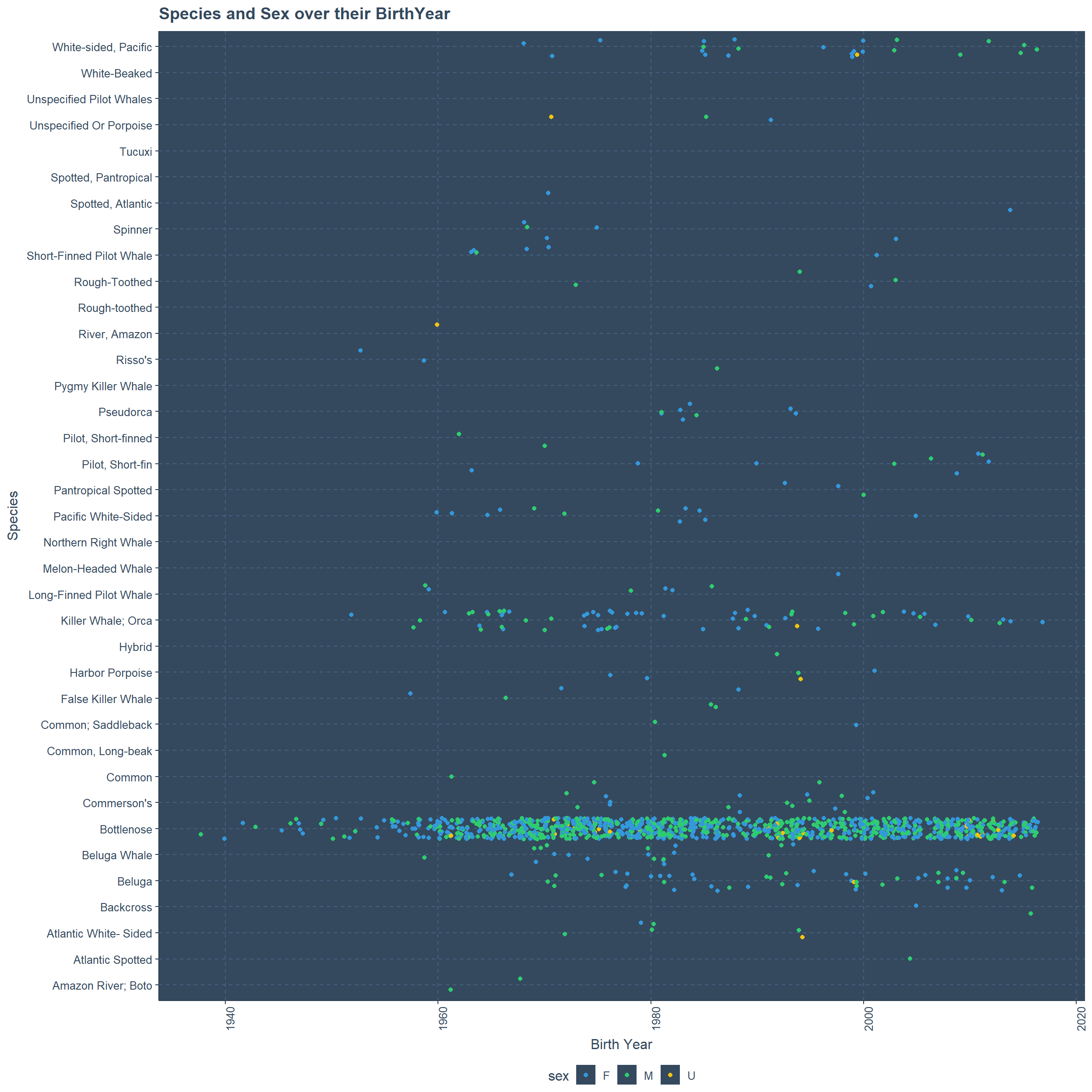

#ggsave("Plot_1.png",width = 12,height = 12)

Species vs Sex vs BirthYear (plot)

• Plot 1
• Alot of Bottle-nose type species from early years.
• More missing values for Birth Year.
• Second most goes to Killer Whale Orca.
• Third place is in with Beluga type Species.
• Here and there few of them without knowledge of Gender.

Status vs Sex vs BirthYear (code)

Plot2<-ggplot(SeaCreature,aes(x=str_wrap(status,8),
                              y=birthYear,color=sex))+
       geom_jitter()+
       coord_flip()+
       theme(axis.text.x =element_text(angle = 90, hjust = 1))+
       ggtitle("Status and Sex over their BirthYear")+
       ylab("Birth Year")+
       xlab("Status")+ 
       legend_bottom()  
Plot2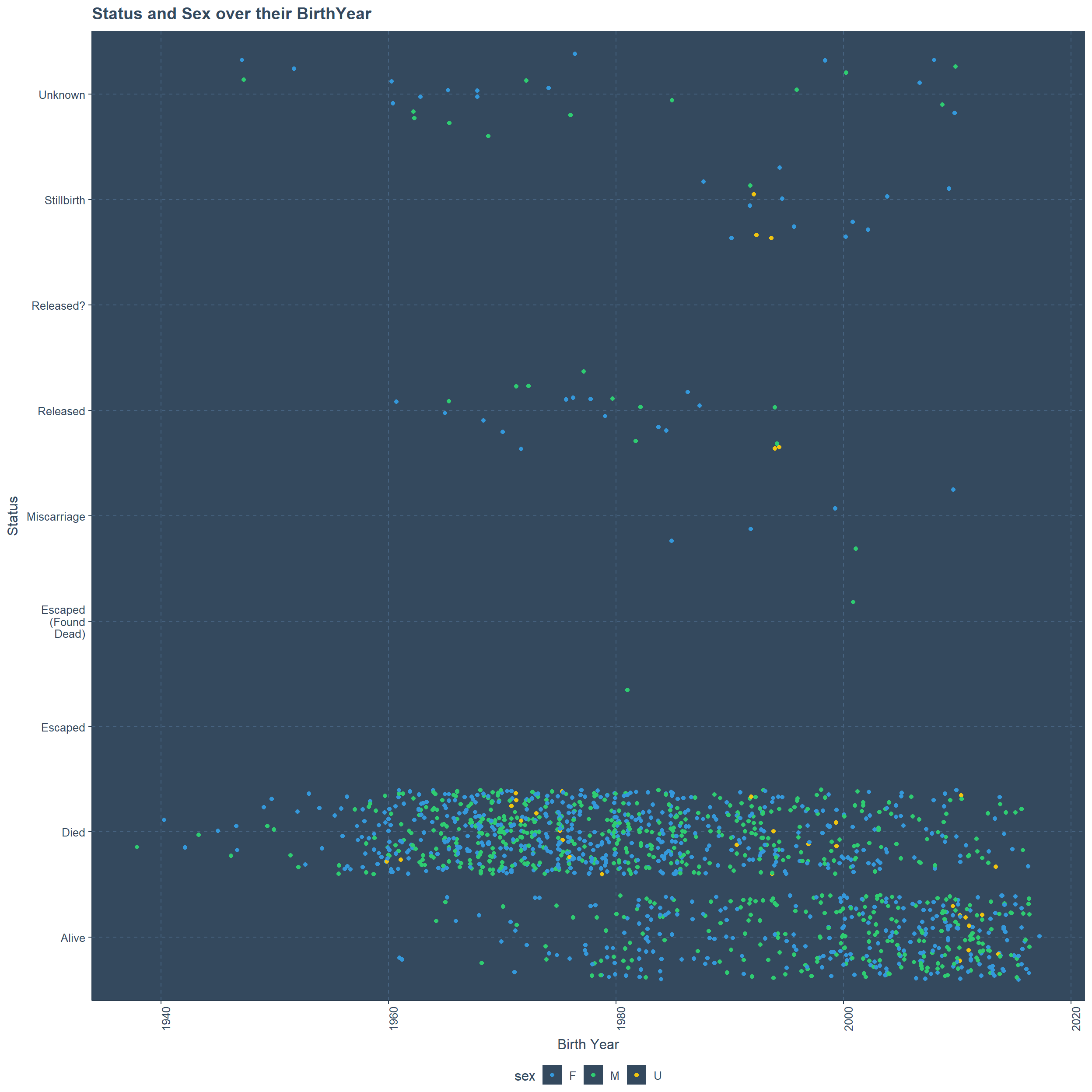

#ggsave("Plot_2.png",width = 12,height = 12)

Status vs Sex vs BirthYear (plot)

• Plot 2
• Dead Sea Creatures from the beginning of time itself.
• Mostly dead, but from 1960 alot of them are alive.
• Birth Year unknown for most of the Dead and few of the Released.
• Quite a few with status unknown.
• Only one escaped and it is a male in 1981.

Species vs Sex vs Status (code)

Plot3<-ggplot(SeaCreature,aes(x=str_wrap(status,8),
                              y=str_wrap(species,12),color=sex))+
       geom_jitter()+
       coord_flip()+
       theme(axis.text.x =element_text(angle = 90, hjust = 1))+
       ggtitle("Species and Sex over their status")+
       ylab("Species")+
       xlab("Status")+ 
       legend_bottom()  
Plot3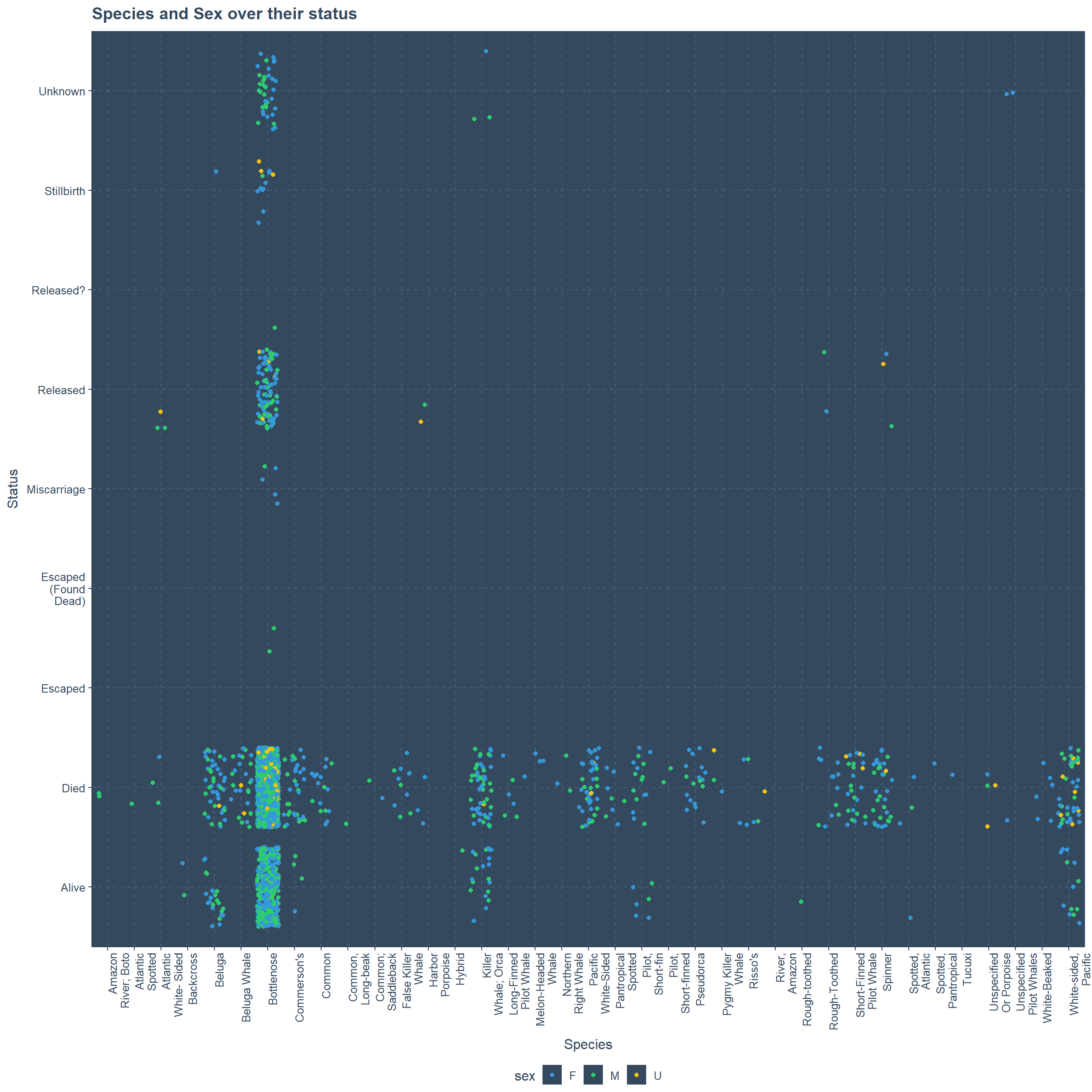

#ggsave("Plot_3.png",width = 14,height = 12)

Species vs Sex vs Status (plot)

• Plot 3
• One male Bottle-nose species escaped.
• More Killer whale orca’s and White-sided Pacific Species are dead than alive
• Around 15 Species have dead creatures and non alive.
• One male Bottle-nose species Escaped but found dead.
• There are 4 miscarriaged Bottle-nose species and three are female.

Birth Year and Sex of the Acquisitioned (code)

Plot4<-ggplot(SeaCreature,aes(x=acquisition,
                              y=birthYear,color=sex))+
       geom_jitter()+
       theme(axis.text.x =element_text(angle = 90, hjust = 1))+
       ggtitle("Acquisitioned ones with their and BirthYear")+
       ylab("Birth Year")+
       xlab("Acquisition")+ 
       legend_bottom()  
Plot4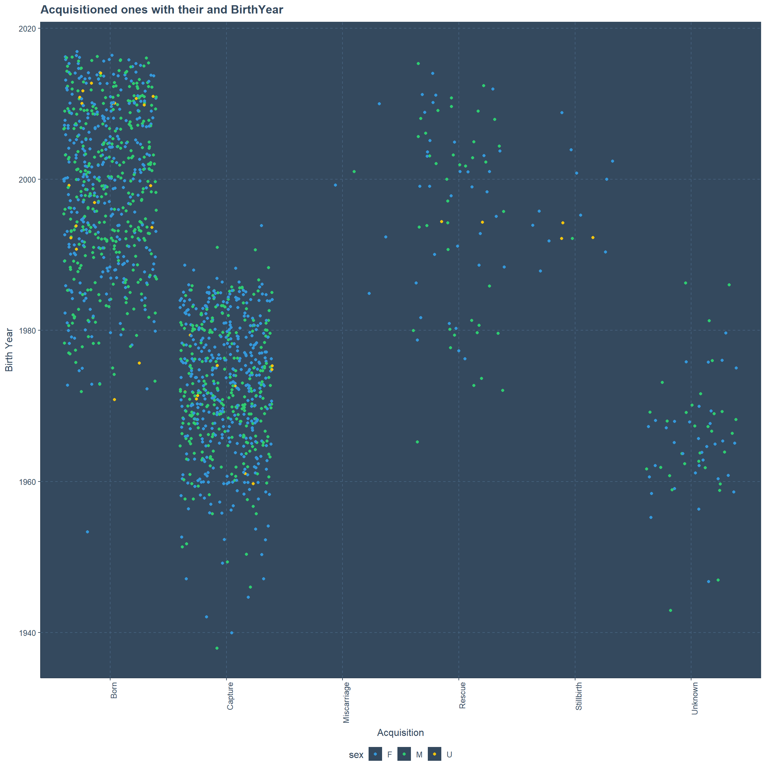

#ggsave("Plot_4.png",width = 12,height = 12)

Birth Year and Sex of the Acquisitioned (plot)

• Plot 4
• With early Birth Year to until 1990 the creatures were captured.
• From Birth Year 1971 to 2017 only the creatures are born.
• After 1965 around 30 creatures have been rescued.
• Close to 40 creatures with unknown status with Birth Year known.
• Most of the rescued ones are of Male gender.

Species and their sex over current location (code)

Plot5<-ggplot(SeaCreature,aes(x=str_wrap(species,12),
                              y=currently,color=sex))+
       geom_jitter()+
       theme(axis.text.x =element_text(angle = 90, hjust = 1))+
       ggtitle("Species and Sex over their Current Location")+
       ylab("Current Location")+
       xlab("Species")+ 
       legend_bottom()  
Plot5

#ggsave("Plot_5.png",width = 14,height = 14)

Species and their sex over current location (plot)

• Plot 5
• Close to 50 current locations.
• There are few locations with only one type of species.
• Bottle-nose creatures in most of these locations.
• Sea Life park in Hawaii has a diverse amount of Species.
• Sea world in San Diego is second when it comes to diversity.

Acquisitioned ones and thier Sex with Status (code)

Plot6<-ggplot(SeaCreature,aes(x=status,y=acquisition,color=sex))+
       geom_jitter()+
       ggtitle("Acquisitioned with Sex and Status")+
       xlab("Status")+
       ylab("Acquisition")+ 
       legend_bottom()  
Plot6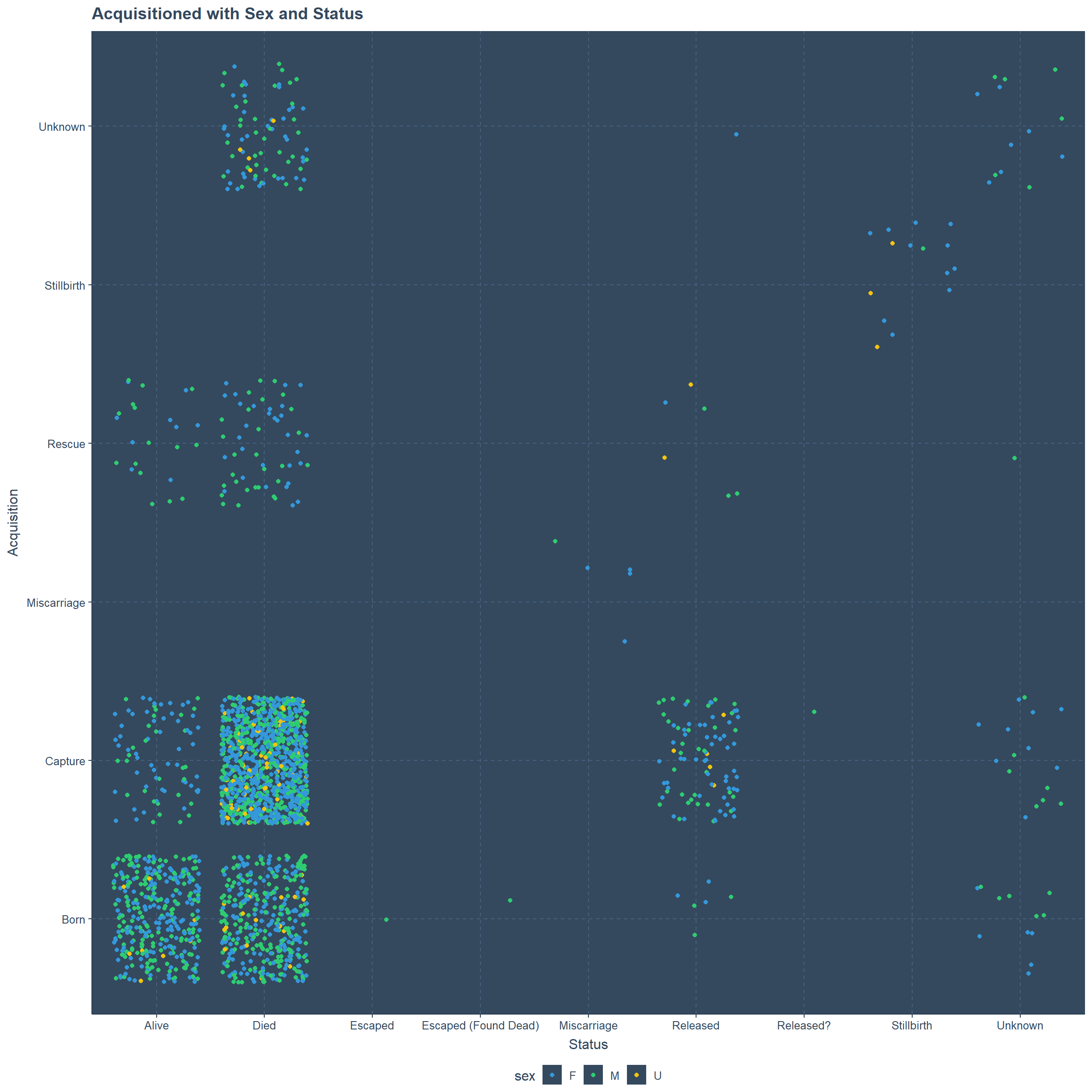

#ggsave("Plot_6.png",width = 12,height = 12)

Acquisitioned ones and thier Sex with Status (plot)

• Plot 6
• Most of the Captured creatures are Dead, but few of them Released.
• Most of the Rescued creatures are Dead, few alive and some Released.
• In Unknown acquisition-ed type alot of them are Dead.
• One rescued creature with unknown status.
• 6 creatures which were born have been released and 50% are male.

Conclusion

• Ios slides are NICE.
• Jitter plots useful for categorical data.
• Plots are too complex when using Location, Currently and Birth Year, but manageable.
• Bottle-nose species is holding a special place in this data-set.
• Alot of unknown data points when it comes to Birth Year.

THANK YOU