Week 8 : Phds Awarded in USA between 2008 and 2017

# load the packages
library(tidyverse)
library(ggthemr)
library(readr)
library(gganimate)
library(ggridges)
library(ggalluvial)

ggthemr("flat")

#load the data
phdlist <- read_csv("phd_by_field.csv")

Five variables are representing this entire data-set and three of them are factors while one column represents the year and the final column is for counts. There are few missing values. We can focus on Phds awarded from 2008 to 2017 in perspective of Broad Field, Major Field and Field.

Dataset

GitHub Code

{{% tweet "1097868689385418752" %}}

Broad Field and Major Field are considered specially but not the column Field as it would be difficult to plot based on the amount of categories.

Broad Field

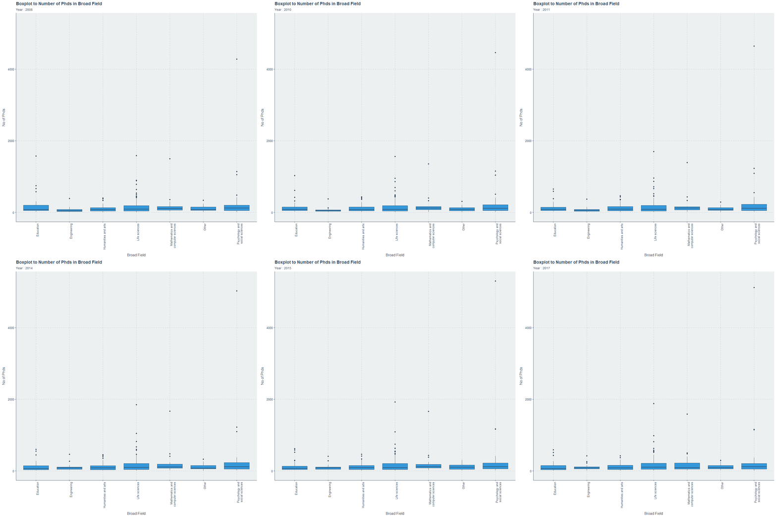
Broad field has 7 categories and clearly Psychology and social sciences has produced more than 4000 Phds each and every year. Which is twice comparing to other categories. If we drop Psychology and Social sciences, now the changes over the years for other categories are clear.

There are more outliers in the field of Life sciences where some programs produce more than 1000 Phds each year comparatively to the rest categories. Except Life sciences other categories tend to behave rarely as above producing more than 1000 Phds.

Engineering field has the lowest distribution with relative to other categories according to the box plot in every year.

All fields

p<-ggplot(phdlist,aes(x=str_wrap(broad_field,20),y=n_phds))+
          geom_boxplot()+
          xlab("Broad Field")+ylab("No of Phds")+
          transition_time(year)+ease_aes("linear")+
          ggtitle("Boxplot to Number of Phds in Broad Field",
              subtitle = "Year : {round(frame_time)}")+
          theme(axis.text.x = element_text(hjust=1,angle = 90))

animate(p,nframes=9,fps=1)

Dropping Psychology and Social Sciences

p<-ggplot(subset(phdlist,broad_field != "Psychology and social sciences"),
          aes(x=str_wrap(broad_field,20),y=n_phds))+
          geom_boxplot()+
          xlab("Broad Field")+ylab("No of Phds")+
          transition_time(year)+ease_aes("linear")+
          ggtitle("Boxplot to Number of Phds in Broad Field",
              subtitle = "Year : {round(frame_time)}")+
          theme(axis.text.x = element_text(hjust=1,angle = 90))

animate(p,nframes=9,fps=1)

Major Field

Focus now solely switches towards the Major Field column and here also we can see the strong outlier in Psychology over the years. Further, Physics and Astronomy field also has a very strong outlier where over the years it reaches 2000 Phds.

Without dropping Psychology we can see the odd behavior from the fields “Education Research”, “Economics” and “Computer and Information Sciences”. Specially the gradual decrease of “Education Research” from 2008 to 2017.

Also in “Computer and Information Sciences” field there is an odd increase in 2012.

After dropping the “Psychology” field we can now clearly see how other Major fields behave over the years.

Major Fields with Box plot

p<-ggplot(phdlist,aes(x=str_wrap(major_field,20),y=n_phds,fill=broad_field))+
          geom_boxplot()+coord_flip()+
          xlab("Major Field")+ylab("No of Phds")+
          transition_time(year)+ease_aes("linear")+
          ggtitle("Boxplot to Number of Phds in Major Field",
              subtitle = "Year : {round(frame_time)}")+
          theme(axis.text.x = element_text(hjust=1,angle = 90),
                legend.position = "bottom")+
          labs(fill="Broad Field")

animate(p,nframes=9,fps=1)

Major Fields without Psychology but still in a Boxplot

q<-ggplot(subset(phdlist,major_field != "Psychology"),
          aes(x=str_wrap(major_field,20),y=n_phds,fill=broad_field))+
          geom_boxplot()+coord_flip()+
          xlab("Major Field")+ylab("No of Phds")+
          transition_time(year)+ease_aes("linear")+
          ggtitle("Boxplot to Number of Phds in Major Field",
              subtitle = "Year : {round(frame_time)}")+
          theme(axis.text.x = element_text(hjust=1,angle = 90),
                legend.position = "bottom")+
          labs(fill="Broad Field")

animate(q,nframes=9,fps=1)

Mathematics and Computer Sciences

I am a Statistics student with a glimpse of Computer science background, therefore my next intention is to focus on the Broad Field “Mathematics and Compute Sciences”.

Mathematics and Computer Science as a Broad field

Mathematics and Statistics has a gradual increase until 2012, but wavers higher and lower in the next years, but in 2016 there is a sudden increase of which would lead to around 700 Phds awarded. Next year this decreases to 500 Phds.

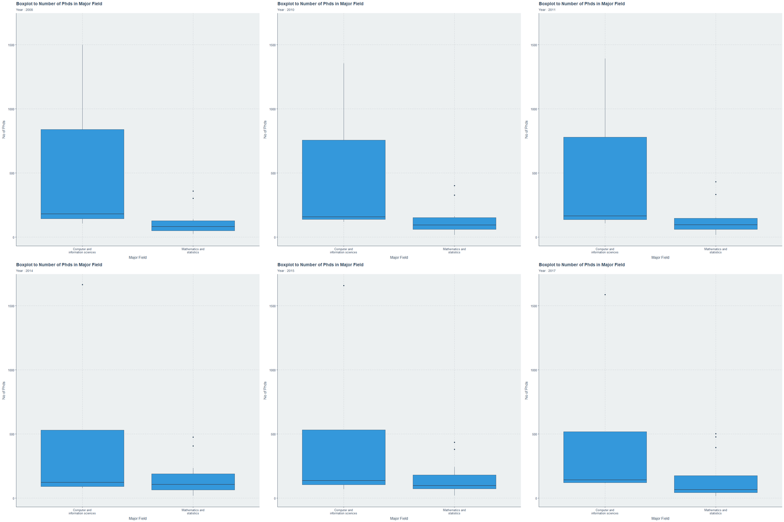
Comparing the 2 major fields “Computer and Information Sciences” with “Mathematics and Statistics” indicate the strong gap between them awarding Phds. “Computer and Information Sciences” award more than twice the amount of Phds what “Mathematics and Statistics” award each year.

“Computer and Information Sciences” also hold a clear pattern with the Phds awarded.

subset(phdlist,broad_field == "Mathematics and computer sciences") %>%
      
ggplot(.,aes(x=factor(year),y=n_phds,fill=major_field))+
       geom_bar(stat="identity",position = "dodge")+
       theme(legend.position = "bottom")+
       xlab("Major Field")+ylab("Number of Phds")+
       ggtitle("Number of Phds awarded under Mathematics and CS",
               subtitle = "Year : 2008 to 2017")+
      scale_y_continuous(breaks=seq(0,1700,100),labels=seq(0,1700,100))+
          labs(fill="Major Field")

Mathematics and Computer Science as a Major Field

Box plot indicates the clear variation among these two major fields over years which could be used for comparison. The sudden peak in year 2012 for “Computer and Information Sciences” interests me alot. It should be noted that “Mathematics and Statistics” has more outliers than “Computer and Information Sciences”.

p<-ggplot(subset(phdlist,broad_field == "Mathematics and computer sciences"),
          aes(x=str_wrap(major_field,20),y=n_phds))+
          geom_boxplot()+
          xlab("Major Field")+ylab("No of Phds")+
          transition_time(year)+ease_aes("linear")+
          ggtitle("Boxplot to Number of Phds in Major Field",
              subtitle = "Year : {round(frame_time)}")

animate(p,nframes=9,fps=1)

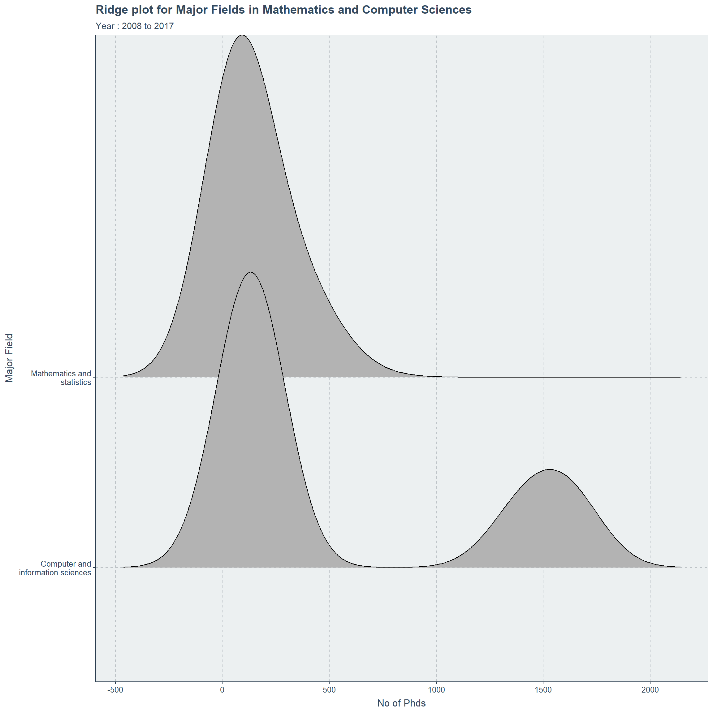
Below is a ridge plot to describe the same thing which would clearly indicate the data spread.

ggplot(subset(phdlist,broad_field == "Mathematics and computer sciences"),
          aes(y=str_wrap(major_field,20),x=n_phds))+
          geom_density_ridges()+
          xlab("No of Phds")+ ylab("Major Field")+
          theme(legend.position = "bottom")+
          ggtitle("Ridge plot for Major Fields in Mathematics and Computer Sciences",
                  subtitle = "Year : 2008 to 2017")

Major Field of Mathematics and Computer Science but now all Fields

Considering the sub categories of the chosen broad field in a box plot did not work quite well, but clearly this plot indicates the Computer Science Phds being awarded with highest amount over the years. Would that mean the boom of Artificial Intelligence in Computer Science.

p<-ggplot(subset(phdlist,broad_field == "Mathematics and computer sciences"),
          aes(x=str_wrap(field,20),y=n_phds,fill=major_field))+
          geom_boxplot()+coord_flip()+
          xlab("Field")+ylab("No of Phds")+
          transition_time(year)+ease_aes("linear")+
          ggtitle("Boxplot to Number of Phds in Field",
              subtitle = "Year : {round(frame_time)}")+
          theme(legend.position = "bottom")+
          labs(fill="Major Field")

animate(p,nframes=9,fps=1)

To get a clear view here is the ridge plot, where Computer Science is very strong for “Computer and Information Sciences”. It should be noted though there is only three other fields in this major field which are “Information Science systems”, “Computer and Information Sciences, other” and “Computer and Information sciences, general”.

More than 10 fields for the Major field “Mathematics and Statistics”, where higher counts occur to “Statistics(Mathematics)”, “Applied mathematics” and “Mathematics and Statistics,general”. Still non of these fields have passed the 1000 Phds awarded mark.

ggplot(subset(phdlist,broad_field == "Mathematics and computer sciences"),
          aes(y=str_wrap(field,20),x=n_phds,fill=major_field))+
          geom_density_ridges()+
          xlab("No of Phds")+ ylab("Field")+
          theme(legend.position = "bottom")+
          ggtitle("Ridge plot for Fields in Mathematics and Computer Sciences",
                  subtitle = "Year : 2008 to 2017")+
          labs(fill="Major Field")

Major Field, Field and Year For Mathematics and Computer Sciences

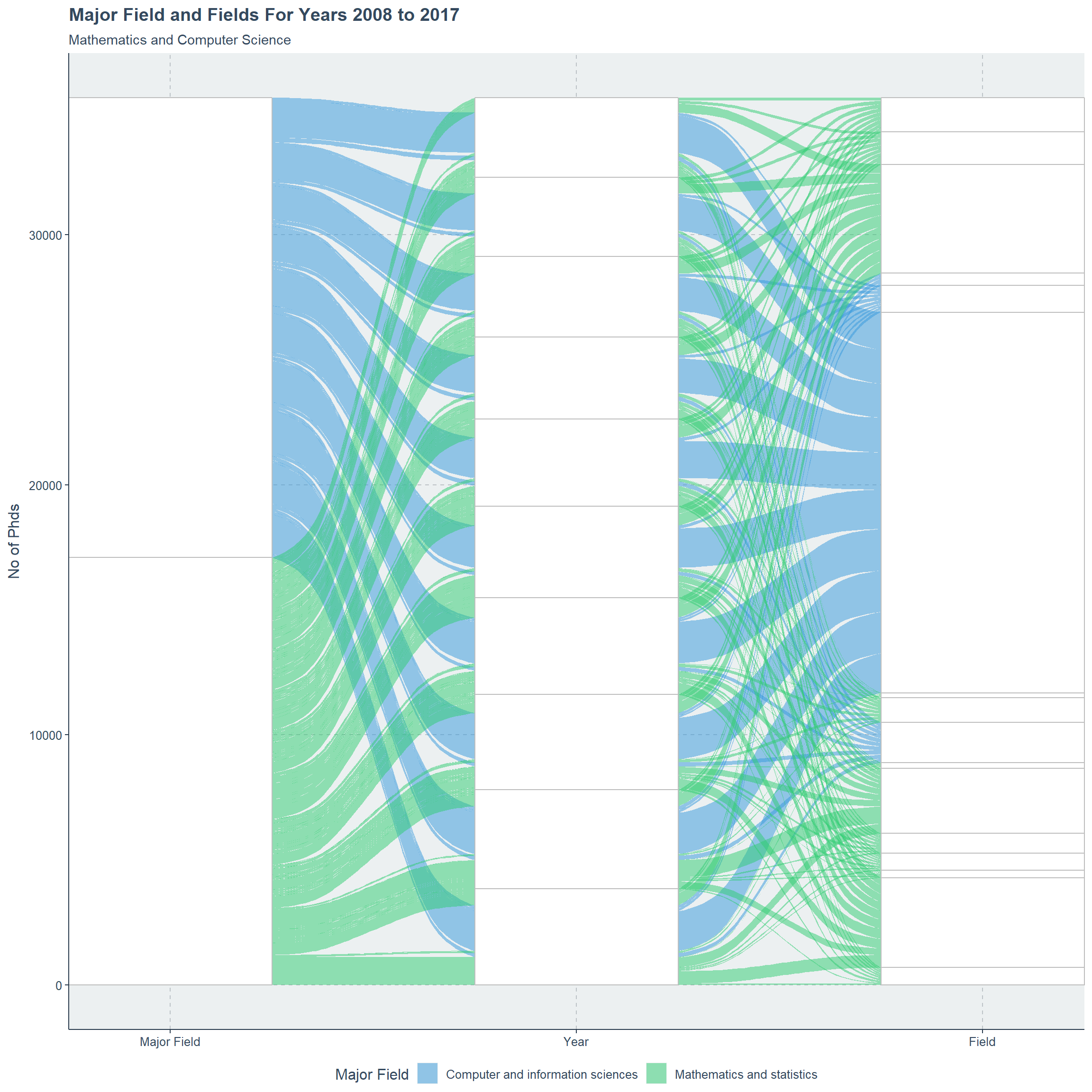
Finally an alluvial diagram just to look at the impact of Computer science field with respective to each year, which is very strong.

data.frame(subset(phdlist,broad_field=="Mathematics and computer sciences")) %>%
           na.omit() %>%
ggplot(.,aes(axis2=factor(str_wrap(year,10)), axis1= factor(str_wrap(major_field,10)), 
             axis3= factor(field), y=as.numeric(n_phds)))+
       scale_x_discrete(limits=c("Major Field","Year","Field"),expand = c(.05, .05))+
       geom_alluvium(aes(fill=factor(major_field)),width = 1/2)+
       geom_stratum(width=1/2,fill="white",color="grey")+
       geom_text(stat = "stratum", label.strata = TRUE)+
       theme(legend.position = "bottom")+ylab("No of Phds")+
       ggtitle("Major Field and Fields For Years 2008 to 2017",
               subtitle="Mathematics and Computer Science")+
          labs(fill="Major Field")

THANK YOU