Week 9 : French Train Delays

# load the packages
library(readr)
library(tidyverse)
library(gganimate)
library(ggalluvial)
library(geomnet)
library(ggthemr)

# load the theme
ggthemr("fresh")

# load the data
small_trains <- read_csv("small_trains.csv")

GitHub Code

Data set

{{% tweet "1101039210298003456" %}}

Network Graph for the French City Trains

Simply drawing a network graph to understand which french cities are mainly urban with capacity to trains arriving and leaving. Cities such as Paris Lyon, Paris Montparnasse, Paris Nord and Paris Est could be cities of concern with much for traffic with related to trains.

ggplot(small_trains,aes(from_id=departure_station,to_id=arrival_station))+
          geom_net(directed = TRUE,labelon = TRUE,size=0.5,labelcolour = "black",
                   repel = FALSE,ecolour = "grey70", arrowsize = 0.75,
                   linewidth = 0.5,layout.alg = "fruchtermanreingold")+
          theme_net()+
          ggtitle("Network Graph Showing from City to City of French Trains")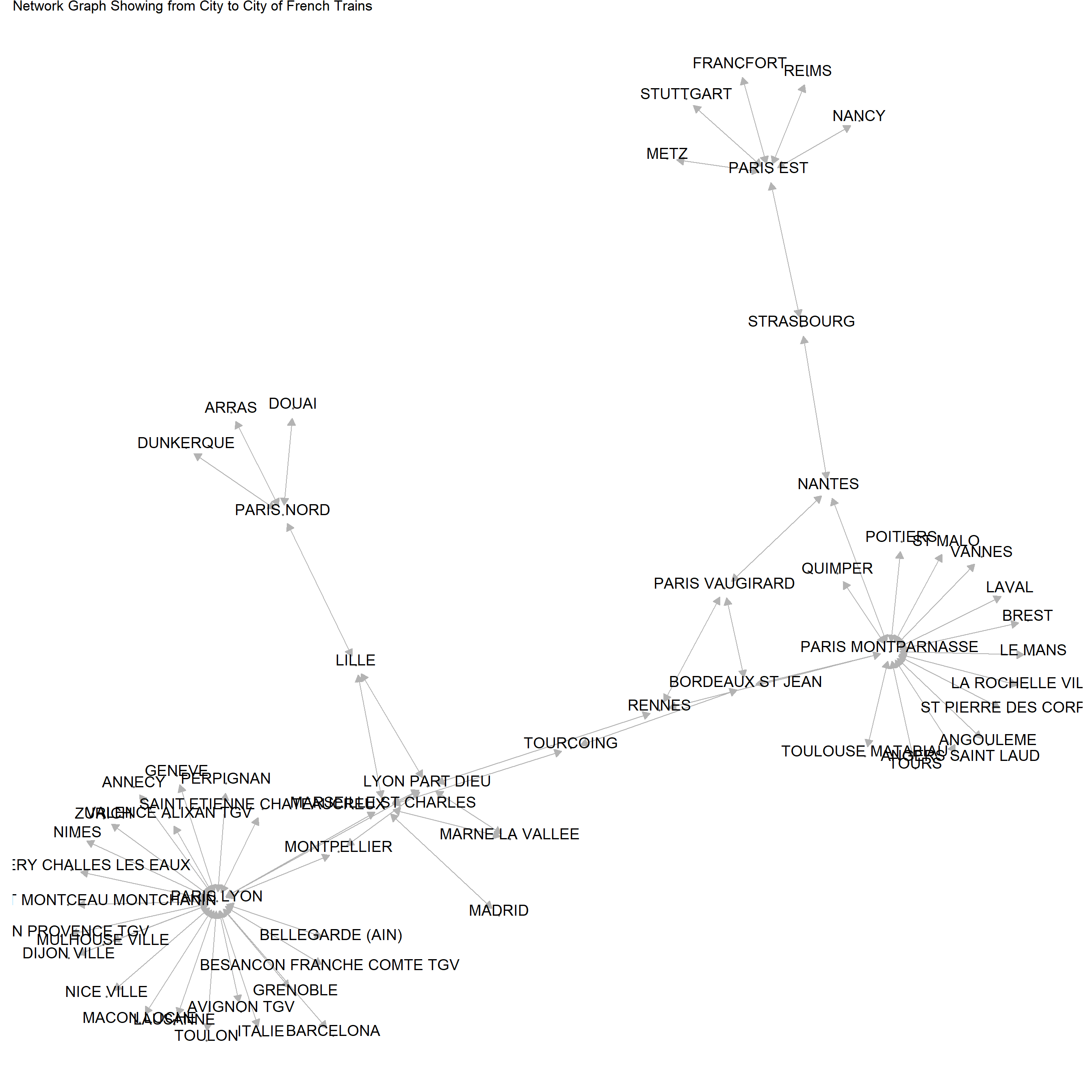

Paris Montparnasse

Let me focus on Montparnasse which has lot of trains coming towards and leaving outwards according to the network map. Not all are cities of France according to my observations, where I can see Madrid, Zurich and Barcelona.

Chosen City with Total Number of Trips

Total number of trips from Paris Montparnasse station to other cities is noted here. Four years of data with more accuracy by months is considered in this plot. There is clear variation in this data for cities.

Close to 800 trips have been recorded towards the Bordeaux St Jean city but not clearly the same pattern for all years or months as well. Further, St Malo city has the lowest amount of trips compared to other cities in all fours but follows a centered pattern around the 100 mark.

p<-ggplot(subset(small_trains,departure_station=="PARIS MONTPARNASSE"),
       aes(x=str_wrap(arrival_station,20),y=total_num_trips,color=month))+
       geom_jitter()+coord_flip()+ labs(color="Month")+
       transition_time(year)+ease_aes("linear")+
       scale_y_continuous(breaks = seq(0,800,100),labels=seq(0,800,100))+
       xlab("Arrival Station")+ylab("Total Number of Trips")+
       ggtitle("Paris Montparnasse and its arrival Stations" ,subtitle ="Year :{frame_time}")

animate(p,nframes=4,fps=1)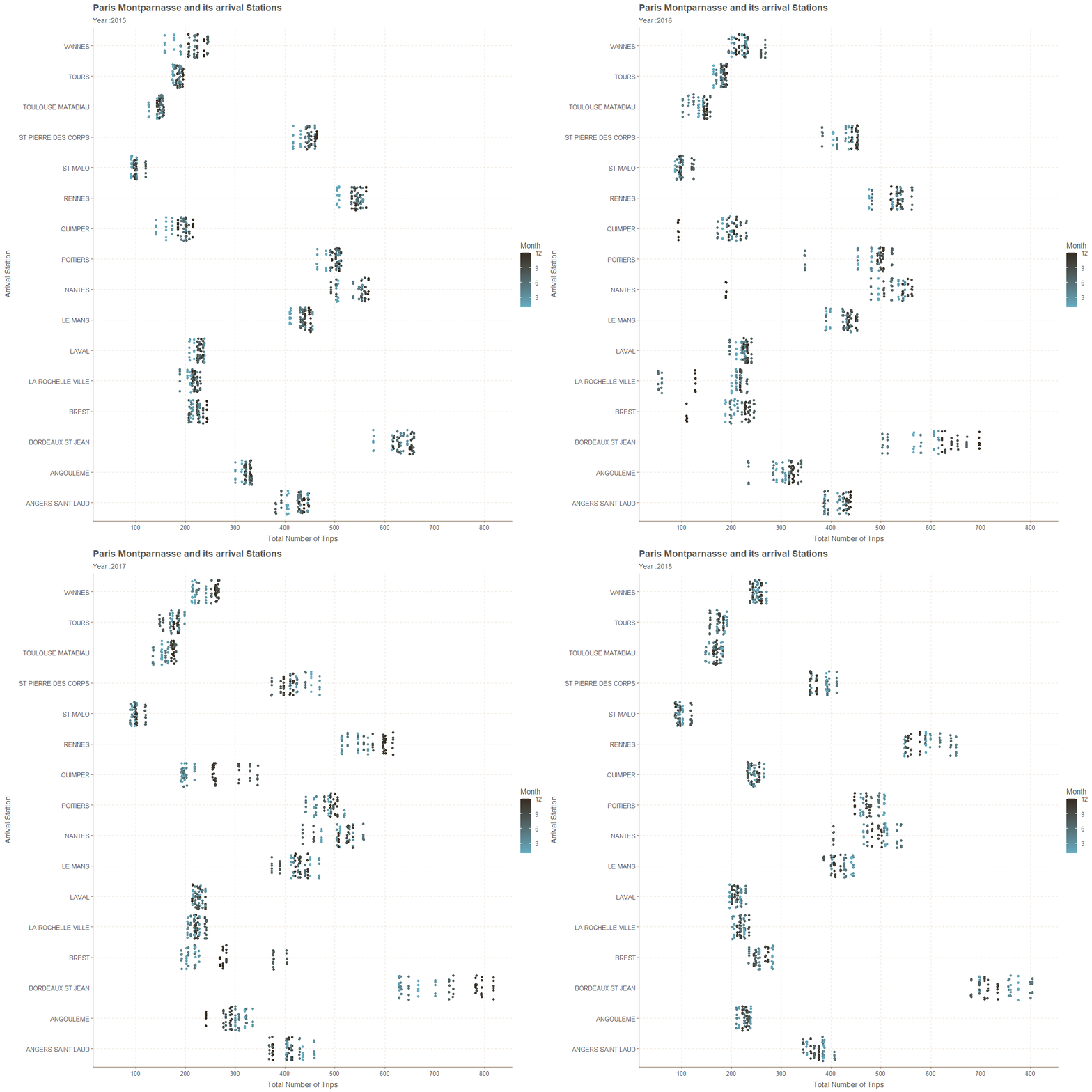

Chosen City with Average Journey Time

Except year 2017 all cities has similar and centered data points. In this exceptional year of 2017 we can see a difference between the first six months and rest. Where most of the Average journey times have been reduced, it is clear according to year 2018 points.

City of Toulouse Matabiau has the highest Average Journey Time, while lowest time goes to the city of Le Mans. So what happened after mid of year 2017.

Maximum Average Journey time before mid of year 2017 is close to 325 but after this period it is centered around 275. The Minimum Average Journey time before mid of year 2017 and after also it is close to 50.

p<-ggplot(subset(small_trains,departure_station=="PARIS MONTPARNASSE"),
       aes(x=str_wrap(arrival_station,20),y=journey_time_avg,color=month))+
       geom_jitter()+coord_flip()+ labs(color="Month")+
       transition_time(year)+ease_aes("linear")+
       scale_y_continuous(breaks=seq(0,350,25),labels=seq(0,350,25))+
       xlab("Arrival Station")+ylab("Average Journey Time")+
       ggtitle("Paris Montparnasse and its arrival Station" ,subtitle ="Year :{frame_time}")

animate(p,nframes=4,fps=1)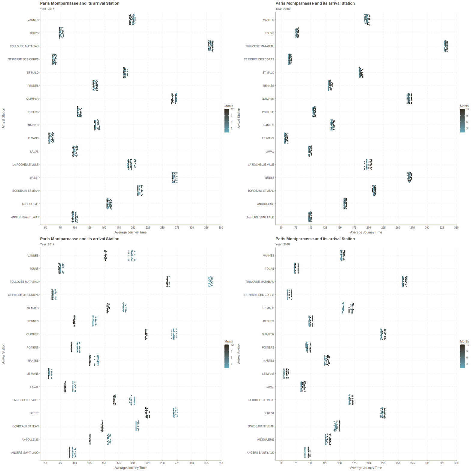

Chosen City with Average Delay with All Departing

There is no clear pattern in perspective of months or years because data points are spread all over the place. Yet there is an odd occurring of negative values for average delay with all departing for some cities after mid of year 2017.

Well none of these negative values does not exceed -2.5, where the maximum average delay in all departing is close to 5.5. I believe unit measured is in minutes.

p<-ggplot(subset(small_trains,departure_station=="PARIS MONTPARNASSE"),
       aes(x=str_wrap(arrival_station,20),y= avg_delay_all_departing,color=month))+
       geom_jitter()+coord_flip()+ labs(color="Month")+
       scale_y_continuous(breaks=seq(-2.5,5.5,0.5),labels=seq(-2.5,5.5,0.5))+
       transition_time(year)+ease_aes("linear")+
       geom_hline(yintercept = 0,color="red")+
       xlab("Arrival Station")+ylab("Average Delay All Departing")+
       ggtitle("Paris Montparnasse and its arrival Station" ,subtitle ="Year :{frame_time}")

animate(p,nframes=4,fps=1)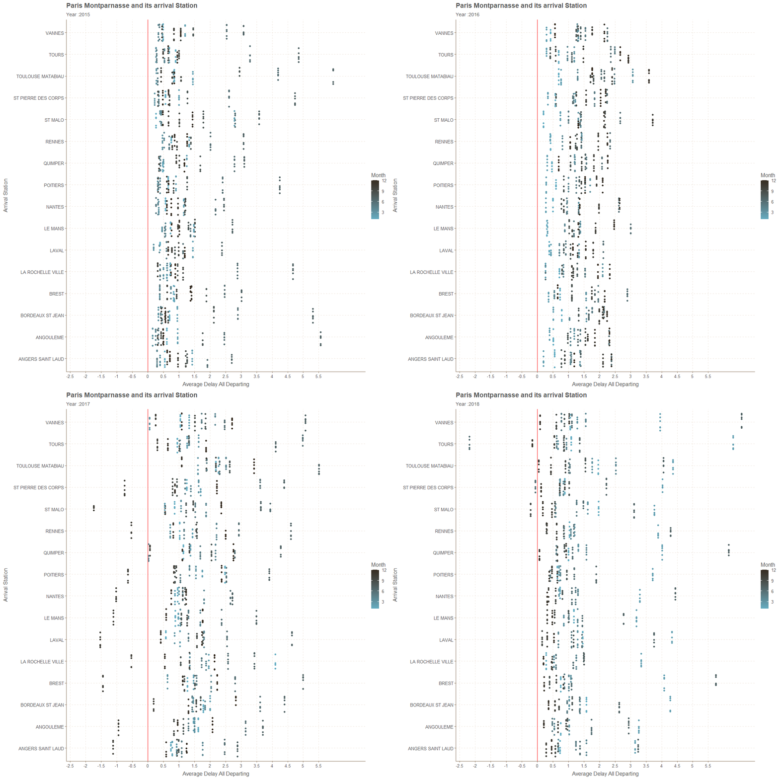

Chosen City with Average Delay with All Arriving

Highest delay could occur close to 18 minutes for average delay in Arriving and the lowest is close to -3. only in 2018 we see such negative values. These negative values occurs for the city of St Malo. Also there is no clear pattern in any city with relative to year or months.

p<-ggplot(subset(small_trains,departure_station=="PARIS MONTPARNASSE"),
       aes(x=str_wrap(arrival_station,20),y=avg_delay_all_arriving,color=month))+
       geom_jitter()+coord_flip()+ labs(color="Month")+
       transition_time(year)+ease_aes("linear")+
       geom_hline(yintercept = 0,color="red")+
       scale_y_continuous(breaks=seq(-3,18),labels=seq(-3,18))+
       xlab("Arrival Station")+ylab("Average Delay All Arriving")+
       ggtitle("Paris Montparnasse and its arrival Station" ,subtitle ="Year :{frame_time}")

animate(p,nframes=4,fps=1)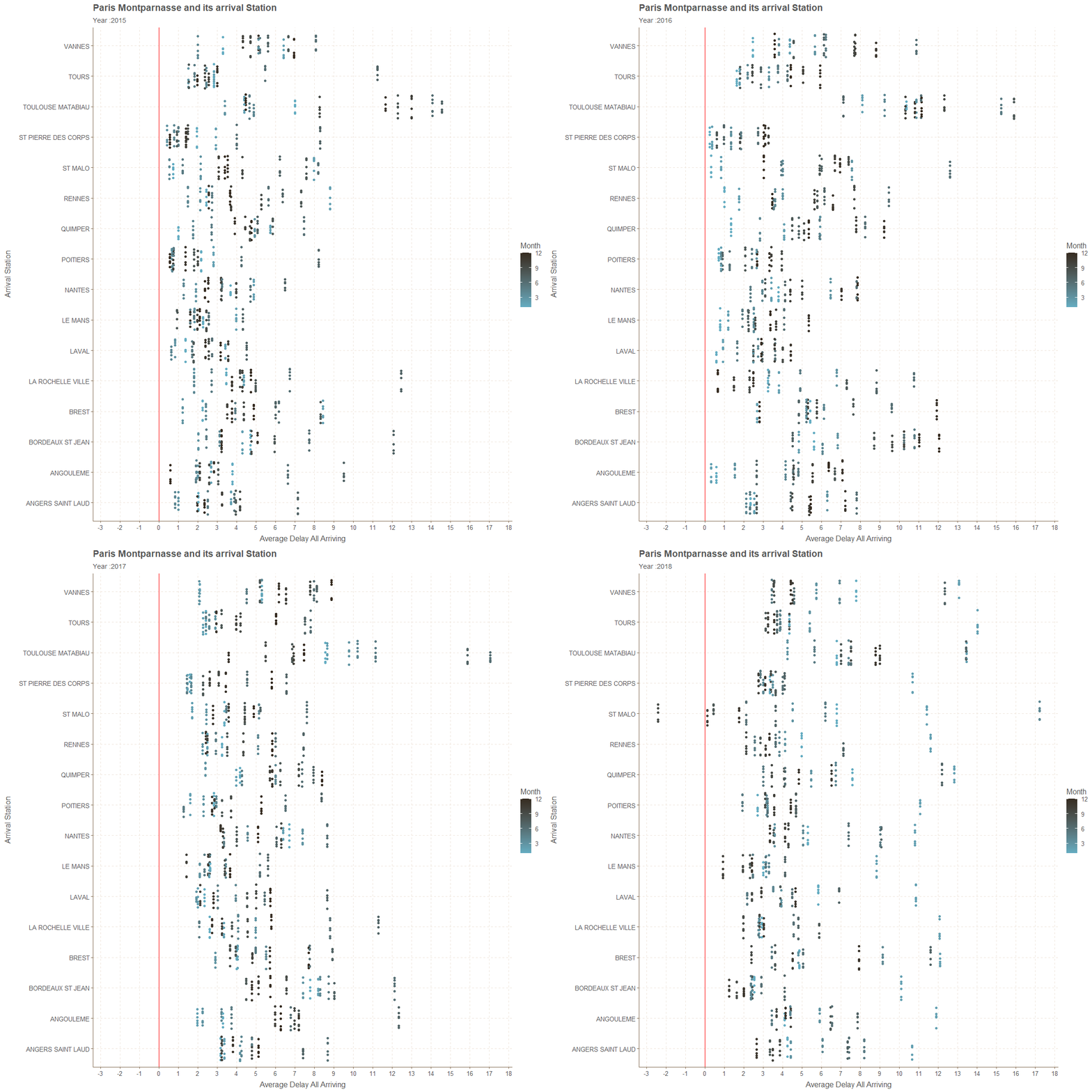

Chosen City with Number of Late Departures

Number of Late departures over the years increases for all cities. It is more clear for Bordeaux St Jean where the counts go beyond 150 and close to 200 in the year of 2018, but in 2015 the highest point is close to 75 for the same city.

St Malo has the lowest number of late departures where it fails to reach the count of 30 in all four years.

p<-ggplot(subset(small_trains,departure_station=="PARIS MONTPARNASSE"),
       aes(x=str_wrap(arrival_station,20),y=num_late_at_departure,
           color=month))+
       geom_jitter()+coord_flip()+ labs(color="Month")+
       scale_y_continuous(breaks=seq(0,200,25),labels=seq(0,200,25))+
       transition_time(year)+ease_aes("linear")+
       xlab("Arrival Station")+ylab("Number of Lates at Departure")+
       ggtitle("Paris Montparnasse and its arrival Station" ,subtitle ="Year :{frame_time}")

animate(p,nframes=4,fps=1)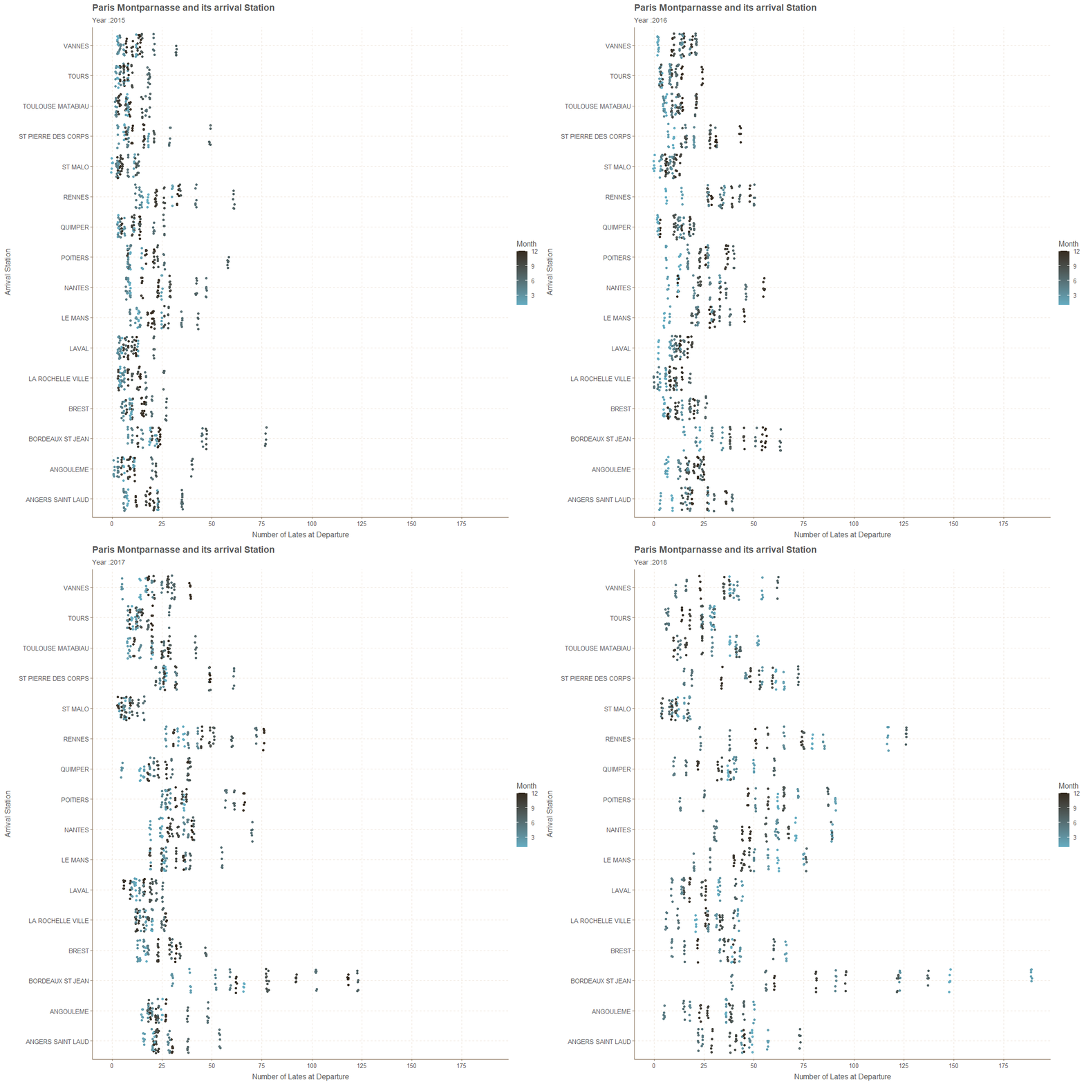

Chosen City with Number of Late Arrivals

City of St Malo has the lowest amount of late arrivals for all fours in general. Most amount of highest late arrivals occur in the city of Bordeaux St Jean. In year 2015 most of these data points are centered towards their specific values. In the next few years we can see that is not the case and they are with a lot of variation.

p<-ggplot(subset(small_trains,departure_station=="PARIS MONTPARNASSE"),
       aes(x=str_wrap(arrival_station,20),y=num_arriving_late,
           color=month))+
       geom_jitter()+coord_flip()+ labs(color="Month")+
       transition_time(year)+ease_aes("linear")+
       scale_y_continuous(breaks=seq(0,200,20),labels=seq(0,200,20))+
       xlab("Arrival Station")+ylab("Number of Lates at Arriving")+
       ggtitle("Paris Montparnasse and its arrival Station" ,subtitle ="Year :{frame_time}")

animate(p,nframes=4,fps=1)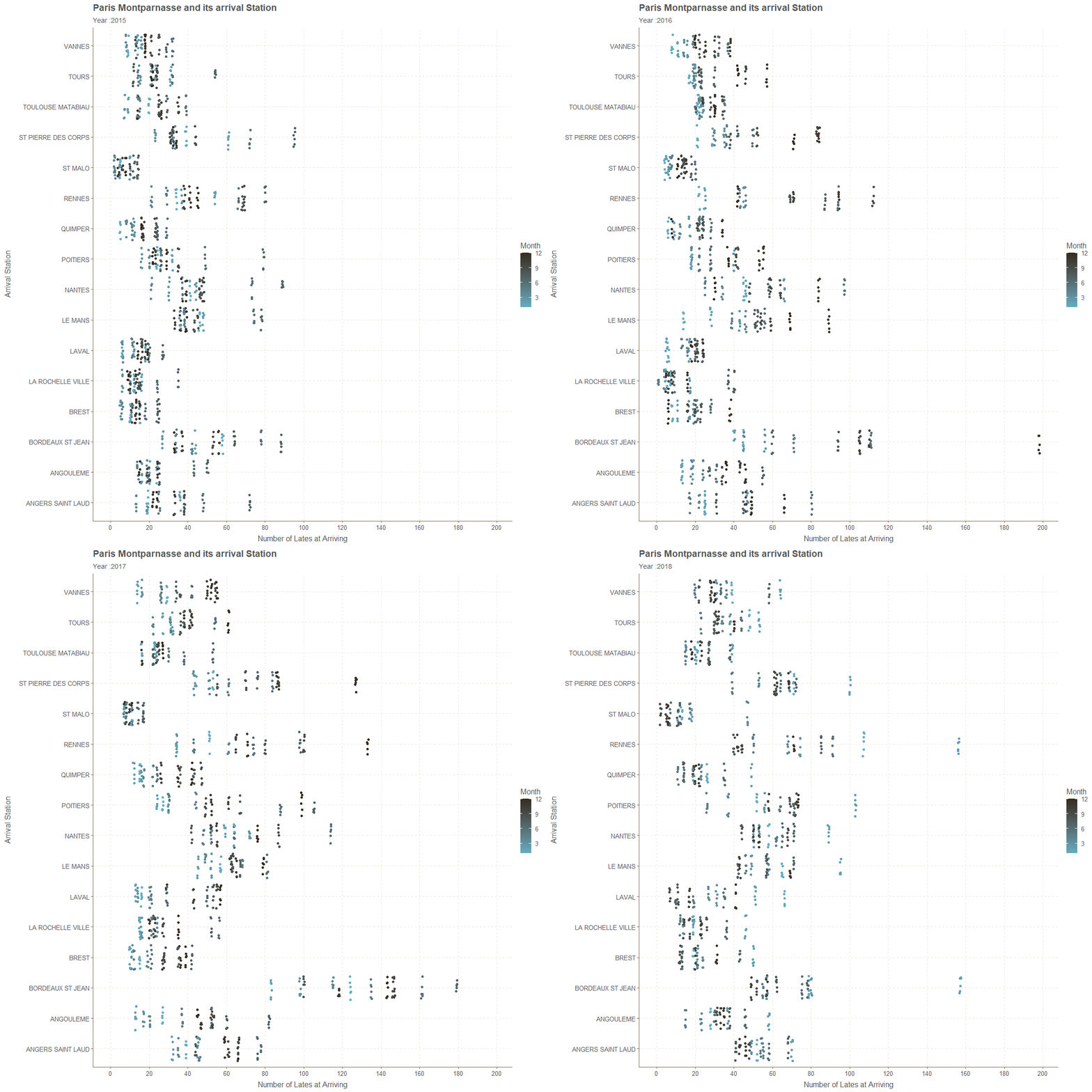

Departure Station with Average Journey Time and Total Number of Trips

Summary of this below plot is that when Average Journey Time increases clearly Total Number of Trips will decrease.

p<-ggplot(small_trains,aes(x=journey_time_avg,y=total_num_trips,color=month))+
      geom_point()+transition_states(departure_station)+labs(color="Month")+
      ggtitle("Average Journey Time and Total Number of Trips",
              subtitle="Departure Station : {closest_state}")+
      scale_y_continuous(breaks=seq(0,900,50),labels=seq(0,900,50))+
      scale_x_continuous(breaks=seq(0,500,50),labels=seq(0,500,50))+  
      xlab("Average Journey Time")+ylab("Total Number of Trips")+
      shadow_mark()

animate(p,nframes=59,fps=1)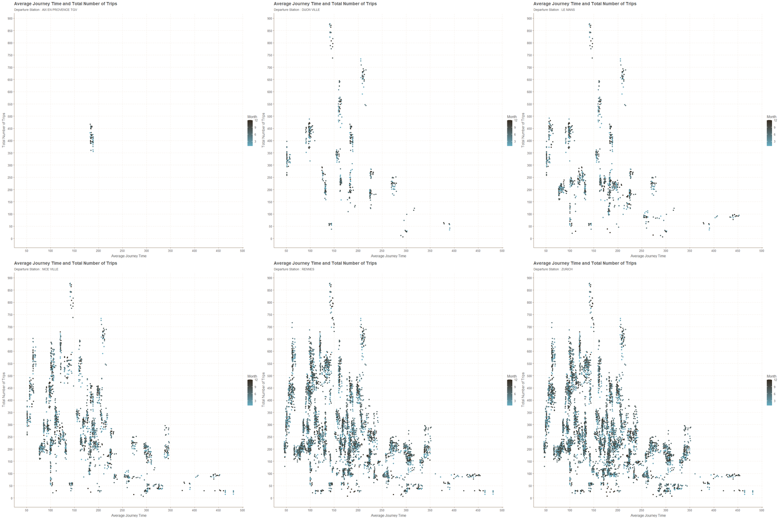

Departure Station with Average Delay All Departing and Number of Late at Departures

p<-ggplot(small_trains,aes(x=num_late_at_departure,y=avg_delay_all_departing,
                           color=month))+
      geom_point()+transition_states(departure_station)+labs(color="Month")+
      ggtitle("Average Delay at All Departing and Number of Lates at Departure",
              subtitle="Departure Station : {closest_state}")+
      geom_vline(xintercept = 0,color="red")+
      geom_hline(yintercept = 0,color="red")+
      scale_y_continuous(breaks=seq(-5,175,5),labels=seq(-5,175,5))+
      scale_x_continuous(breaks=seq(0,500,50),labels=seq(0,500,50))+  
      xlab("Number of Lates at Departure")+ylab("Average Delays at all Departing")+
      shadow_mark()

animate(p,nframes=59,fps=1)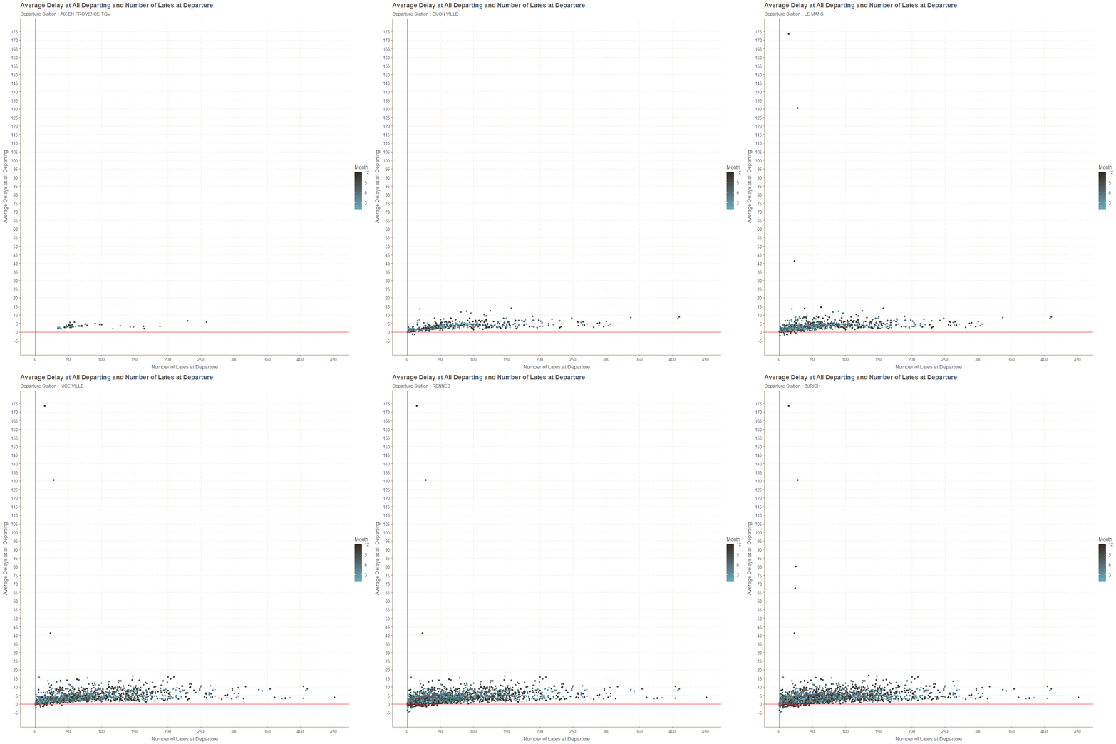

Departure Station with Average Delay All Arriving and Number of Arriving Late

p<-ggplot(small_trains,aes(x=num_arriving_late,y=avg_delay_all_arriving,
                           color=month))+
      geom_point()+transition_states(departure_station)+labs(color="Month")+
      ggtitle("Average Delay at All Arriving and Number of Lates at Arriving",
              subtitle="Departure Station : {closest_state}")+
      geom_vline(xintercept = 0,color="red")+
      geom_hline(yintercept = 0,color="red")+
      scale_y_continuous(breaks=seq(-150,40,5),labels=seq(-150,40,5))+
      scale_x_continuous(breaks=seq(0,250,25),labels=seq(0,250,25))+  
      xlab("Number of Lates at Arriving")+ylab("Average Delays at all Arriving")+
      shadow_mark()

animate(p,nframes=59,fps=1)

Delayed Cause and Delayed Number

Delays caused by the travelers is very less likely to happen, where most of these delays are caused by external causes. Other causes such as rolling stock and rail infrastructure also has effect but not as much from external cause. Station management has limited amount of affect but higher than travelers in causes for delaying trains.

small_trains %>%
    mutate(delay_cause = str_remove(delay_cause,"delay_cause_")) %>%
ggplot(.,aes(x=delay_cause,y=delayed_number))+
      xlab("Delay Cause")+ylab("Delayed Number")+
      ggtitle("Delayed Causes and Delayed Number as percentage")+
      geom_jitter()+coord_flip()

THANK YOU